Joe Biden's Approval Margins

Create a plot

We are going to use the above data to calculate the average net approval rate (approve - disapprove) for each week since Joe Biden got into office. We will plot the net approval, along with its 95% confidence interval. There are various dates given for each poll, but we will plot up to - enddate, i.e., the date the poll ended.

#We begin by preparing the dataset

#We calculate the net approval at a point in time as a function of the approval and the disapproval
approval_polllist$enddate <- mdy(approval_polllist$enddate)
new_approval <- approval_polllist %>% 
  filter(subgroup=="Voters") %>% 
  mutate(net_approve = approve - disapprove, year = year(enddate), week = week(enddate))

glimpse(new_approval)

## Rows: 383
## Columns: 25
## $ president           <chr> "Joseph R. Biden Jr.", "Joseph R. Biden Jr.", "Jos…
## $ subgroup            <chr> "Voters", "Voters", "Voters", "Voters", "Voters", …
## $ modeldate           <chr> "9/20/2021", "9/20/2021", "9/20/2021", "9/20/2021"…
## $ startdate           <chr> "2/2/2021", "2/4/2021", "2/3/2021", "2/5/2021", "2…
## $ enddate             <date> 2021-02-04, 2021-02-06, 2021-02-07, 2021-02-07, 2…
## $ pollster            <chr> "Rasmussen Reports/Pulse Opinion Research", "RMG R…
## $ grade               <chr> "B", "B-", "B", "B", "B", "B+", "B", "B+", "B", "B…
## $ samplesize          <dbl> 1500, 1200, 1500, 1986, 1500, 1306, 1500, 938, 150…
## $ population          <chr> "lv", "rv", "lv", "rv", "lv", "rv", "lv", "rv", "l…
## $ weight              <dbl> 0.3381875, 0.8806739, 0.1776436, 1.0076223, 0.5016…
## $ influence           <dbl> 0, 0, 0, 0, 0, 0, 0, 0, 0, 0, 0, 0, 0, 0, 0, 0, 0,…
## $ approve             <dbl> 49, 60, 50, 59, 51, 53, 51, 60, 50, 52, 53, 57, 53…
## $ disapprove          <dbl> 48, 32, 47, 35, 46, 40, 47, 40, 47, 45, 43, 35, 44…
## $ adjusted_approve    <dbl> 51.53864, 59.21127, 52.53864, 56.89185, 53.53864, …
## $ adjusted_disapprove <dbl> 42.70779, 33.57311, 41.70779, 36.07688, 40.70779, …
## $ multiversions       <chr> NA, NA, NA, NA, NA, NA, NA, NA, NA, NA, NA, NA, NA…
## $ tracking            <lgl> TRUE, NA, TRUE, NA, TRUE, NA, TRUE, NA, TRUE, TRUE…
## $ url                 <chr> "https://www.rasmussenreports.com/public_content/p…
## $ poll_id             <dbl> 74347, 74354, 74349, 74351, 74352, 74360, 74359, 7…
## $ question_id         <dbl> 139654, 139679, 139669, 139673, 139675, 139698, 13…
## $ createddate         <chr> "2/5/2021", "2/9/2021", "2/8/2021", "2/8/2021", "2…
## $ timestamp           <chr> "13:32:13 20 Sep 2021", "13:32:13 20 Sep 2021", "1…
## $ net_approve         <dbl> 1, 28, 3, 24, 5, 13, 4, 20, 3, 7, 10, 22, 9, 18, 1…
## $ year                <dbl> 2021, 2021, 2021, 2021, 2021, 2021, 2021, 2021, 20…
## $ week                <dbl> 5, 6, 6, 6, 6, 6, 6, 6, 6, 6, 7, 7, 7, 7, 7, 7, 7,…

#We then calculate the 95% CI for average approval margin. This is done using the standard error which is also calculated below. 

margin_ci <- new_approval %>% 
  group_by(week) %>% 
  summarise(avg_approval_margin = mean(net_approve),
            sd_margin = sd(net_approve, na.rm=TRUE),
            count_margin = n(),
            se_margin = sd_margin / sqrt(count_margin),
            ci_margin_up = avg_approval_margin + qt(.975, count_margin-1)*se_margin ,
            ci_margin_dw = avg_approval_margin - qt(.975, count_margin-1)*se_margin
            )

## Warning in qt(0.975, count_margin - 1): NaNs produced

## Warning in qt(0.975, count_margin - 1): NaNs produced

glimpse(margin_ci)

## Rows: 34
## Columns: 7
## $ week                <dbl> 5, 6, 7, 8, 9, 10, 11, 12, 13, 14, 15, 16, 17, 18,…
## $ avg_approval_margin <dbl> 1.000000, 11.888889, 12.846154, 11.666667, 9.28571…
## $ sd_margin           <dbl> NA, 9.778093, 8.404822, 9.492687, 7.936562, 6.9429…
## $ count_margin        <int> 1, 9, 13, 13, 14, 12, 11, 15, 10, 8, 15, 14, 14, 1…
## $ se_margin           <dbl> NA, 3.259364, 2.331078, 2.632798, 2.121135, 2.0042…
## $ ci_margin_up        <dbl> NaN, 19.404997, 17.925137, 17.403040, 13.868149, 1…
## $ ci_margin_dw        <dbl> NaN, 4.37278093, 7.76717100, 5.93029320, 4.7032800…

Now we can plot the average approval margin for Joe Biden over the course of his time in office. We do so with the confidence intervals attached. We also plot a line at margin=zero, this allows us to clearly see the points at which Biden moves from a net positive to a net negative approval margin. A line of best flit is plotted in blue

#Plot the for average approval margin
margin_ci %>% 
  ggplot(aes(week)) +
  geom_ribbon(aes(ymin = ci_margin_up, ymax = ci_margin_dw), fill="grey", alpha = 0.5)+
  geom_line(aes(y=avg_approval_margin, group=1), color = "red", size = 0.3) +
  geom_point(aes(y=avg_approval_margin, group=1), color = "red", size  = 0.3) +
  geom_smooth(aes(y=avg_approval_margin)) +
  geom_line(aes(y=ci_margin_up, group=1), color="red", size = 0.3)+
  geom_line(aes(y=ci_margin_dw, group=1), color="red", size = 0.3)+
  
  #add the aesthetics for the graph
  geom_hline(yintercept=0, linetype="solid", color = "orange", size = 1)+
  labs(title="Estimating Approval Margin (Approve-Disapprove) for Joe Biden",
       subtitle = "Weekly average of all polls",
       x = "Week of the Year", 
       y = "Average Approval Margin (Approve - Disapprove)") +
  annotate("text", x = 20, y = 20, label = "2021", color = 'black',size = 3)+
  scale_y_continuous(
    labels = scales::number_format(accuracy = 0.1))+
  theme_minimal()+
  NULL

## `geom_smooth()` using method = 'loess' and formula 'y ~ x'

## Warning: Removed 1 row(s) containing missing values (geom_path).

## Warning: Removed 1 row(s) containing missing values (geom_path).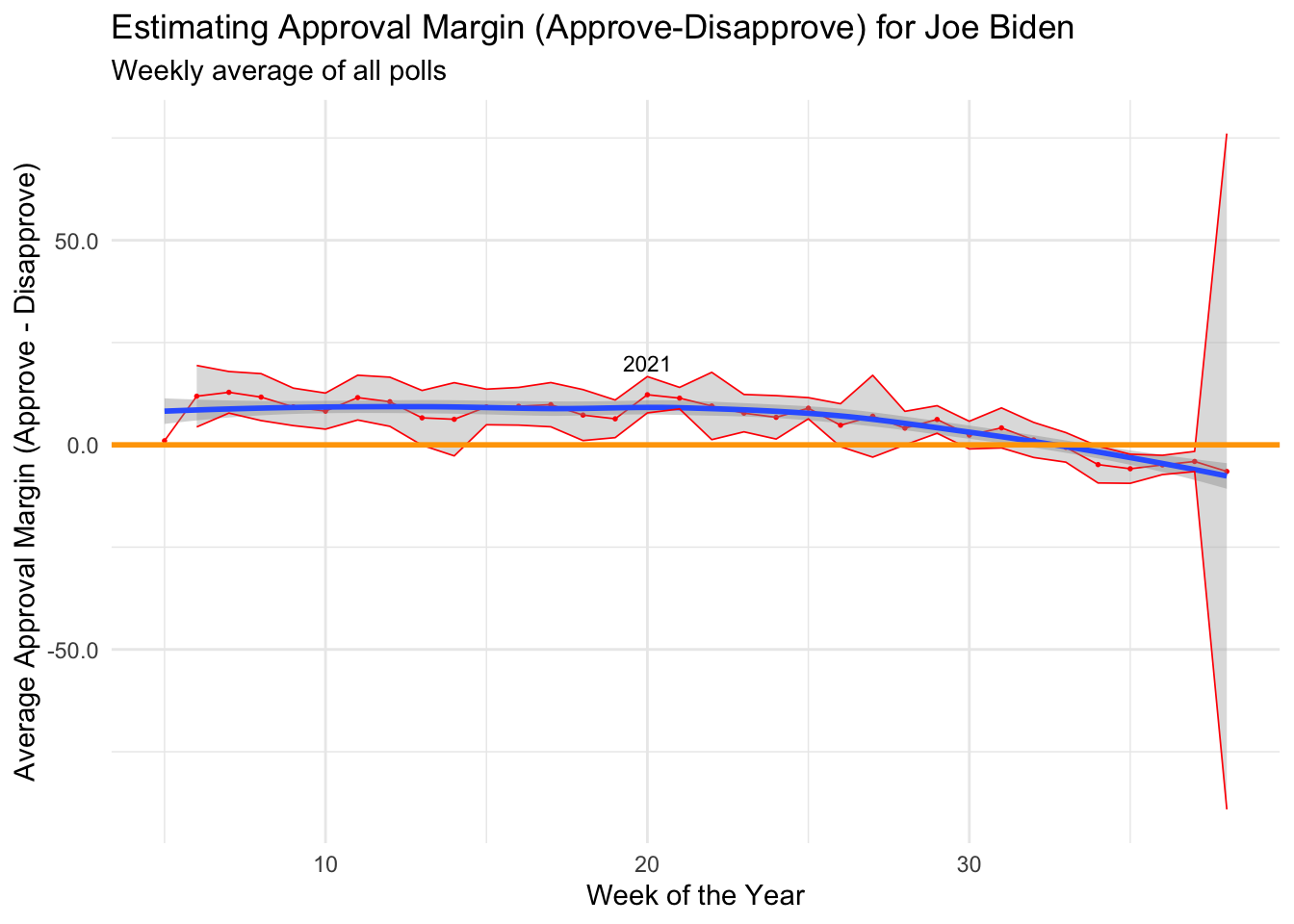

Here, we can see that Biden was able to maintain a fairly positive approval rating for his 30 weeks in office. However, our confidence intervals suggest that there is a possibility that his net approval rating might have been negative at points during this first 30 weeks.

Over the course of the last 5 weeks, we can see that Biden’s net approval margin has become negative, likely as a result of his response to conflicts in Afghanistan. Notably, the confidence interval for the most recent data point is huge, but this is likely to be the result of insufficient data, as supposed to a genuinely large spread of results.