The General Social Survey

The General Social Survey (GSS) gathers data on American society in order to monitor and explain trends in attitudes, behaviours, and attributes. Many trends have been tracked for decades, so one can see the evolution of attitudes, etc. in American Society. This dataset is particularly useful when it comes to gauging and comparing the usage of technology and social media. This will be the primary focus of this section.
gss <- read_csv("../../data/smallgss2016.csv",
                na = c("", "Don't know",
                       "No answer", "Not applicable"))
## Rows: 2867 Columns: 7## ── Column specification ────────────────────────────────────────────────────────
## Delimiter: ","
## chr (7): emailmin, emailhr, snapchat, instagrm, twitter, sex, degree##
## ℹ Use `spec()` to retrieve the full column specification for this data.
## ℹ Specify the column types or set `show_col_types = FALSE` to quiet this message.Instagram and Snapchat, by sex
Firstly, we use the GSS data to deduce the proportion of people that use Snapchat or Instagram. This proportion is calculated for males and females and also incorporates the calculation of confidence intervals. The question we are trying to answer is as follows:
“Can we estimate the population proportion of Snapchat or Instagram users in 2016?”
The following tasks were completed as part of this analysis.:
Create a new variable,
snap_instathat is Yes if the respondent reported using any of Snapchat (snapchat) or Instagram (instagrm), and No if not. If the recorded value was NA for both of these questions, the value in your new variable should also be NA.Calculate the proportion of Yes’s for
snap_instaamong those who answered the question, i.e. excluding NAs.Using the CI formula for proportions, please construct 95% CIs for men and women who used either Snapchat or Instagram
# Question 1
# This question is completed by mutating the data frame to assign a new variable via logical operation.
temp_gss <- gss %>%
   mutate(snap_insta = case_when(
    snapchat == "Yes" | instagrm == "Yes" ~ "Yes",
    snapchat == "NA" | instagrm == "NA" ~ "NA",
    TRUE ~ "No"
  ))
# Question 2
# This question is completed by filtering out N/A results, and subsequently counting occurences of snap_insta (these are mutated to determine the proportion of users).
prop_gss <- temp_gss %>%
filter(snap_insta != "NA") %>%
count(snap_insta) %>%
mutate(prop = n/sum(n))
colnames(prop_gss) = c("Snapchat or Instagram", "Number", "Proportion [%]")
prop_gss## # A tibble: 2 × 3
## `Snapchat or Instagram` Number `Proportion [%]`
## <chr> <int> <dbl>
## 1 No 858 0.625
## 2 Yes 514 0.375# Question 3
# This question is completed by grouping by 'sex' and then calculate n, the standard deviation and the standard error to allow for calculation of the confidence intervals.
CI_gss2 <- temp_gss %>%
filter(snap_insta != "NA") %>%
mutate(snap_insta = snap_insta == "Yes") %>%
group_by(sex) %>%
summarise(Mean_Proportion = mean(snap_insta),
SD_Proportion = sd(snap_insta),
Count_Proportion = n(),
Standard_Error_Proportion = SD_Proportion / sqrt(Count_Proportion),
Upper_CI_Proportion = Mean_Proportion + qt(.975, Count_Proportion-1)*Standard_Error_Proportion ,
Lower_CI_Proportion = Mean_Proportion - qt(.975, Count_Proportion-1)*Standard_Error_Proportion
)
CI_gss2## # A tibble: 2 × 7
## sex Mean_Proportion SD_Proportion Count_Proportion Standard_Error_Proporti…
## <chr> <dbl> <dbl> <int> <dbl>
## 1 Female 0.419 0.494 769 0.0178
## 2 Male 0.318 0.466 603 0.0190
## # … with 2 more variables: Upper_CI_Proportion <dbl>, Lower_CI_Proportion <dbl>The 95% confidence intervals for males and females above do not overlap. Therefore, we can say with reasonable certainty that a larger proportion of females use snapchat or instagram than males.
Twitter, by education level
Secondly, we can use the GSS data to estimate the proportion of people that use twitter at different levels of education.
“Can we estimate the population proportion of Twitter users by education level in 2016?”
This will be done with reference to the following tasks:
Turn
degreefrom a character variable into a factor variable. Make sure the order is the correct one and that levels are not sorted alphabetically which is what R by default does.Create a new variable,
bachelor_graduatethat is Yes if the respondent has either aBachelororGraduatedegree. As before, if the recorded value for either was NA, the value in your new variable should also be NA.Calculate the proportion of
bachelor_graduatewho do (Yes) and who don’t (No) use twitter.Using the CI formula for proportions, please construct two 95% CIs for
bachelor_graduatevs whether they use (Yes) and don’t (No) use twitter.Do these two Confidence Intervals overlap?
#Question 1 - Change 'degree' from character variable to factor variable.
#Levels not sorted alphabetically...

#This task can be completed with simple re-assignment, as shown below...

gss2 <- gss
gss2$degree[gss2$degree == "Lt high school"] <- '1'
gss2$degree[gss2$degree == "High school"] <- '2'
gss2$degree[gss2$degree == "Junior college"] <- '3'
gss2$degree[gss2$degree == "Bachelor"] <- '4'
gss2$degree[gss2$degree == "Graduate"] <- '5'

gss2$degree <- as_factor(gss2$degree)

#We can see the new variable created below...
head(gss2,5)
## # A tibble: 5 × 7
## emailmin emailhr snapchat instagrm twitter sex degree
## <chr> <chr> <chr> <chr> <chr> <chr> <fct>
## 1 0 12 NA NA NA Male 4
## 2 30 0 No No No Male 2
## 3 NA NA No No No Male 4
## 4 10 0 NA NA NA Female 2
## 5 NA NA Yes Yes No Female 5#Question 2 - Create New Variable - 'bachelor_graduate'
#We create the new variable using logical operators:
gss3 <- gss %>%
mutate(bachelor_graduate = case_when(
degree == 'Bachelor' | degree == 'Graduate' ~ "*Yes*",
degree == "NA" ~ "NA",
TRUE ~ "*No*"
))
head(gss3,5)## # A tibble: 5 × 8
## emailmin emailhr snapchat instagrm twitter sex degree bachelor_gradua…
## <chr> <chr> <chr> <chr> <chr> <chr> <chr> <chr>
## 1 0 12 NA NA NA Male Bachelor *Yes*
## 2 30 0 No No No Male High school *No*
## 3 NA NA No No No Male Bachelor *Yes*
## 4 10 0 NA NA NA Female High school *No*
## 5 NA NA Yes Yes No Female Graduate *Yes*#Question 3 - Calculate the proportion of bachelor_graduate that do and do not use twitter...
gss_twitter_prop <- gss3 %>%
filter(bachelor_graduate == "*Yes*") %>%
filter(twitter != "NA") %>%
count(twitter) %>%
mutate(Proportion = n/sum(n) * 100)
colnames(gss_twitter_prop) = c("Twitter", "Number", "Proportion [%]")
print(gss_twitter_prop)## # A tibble: 2 × 3
## Twitter Number `Proportion [%]`
## <chr> <int> <dbl>
## 1 No 375 76.7
## 2 Yes 114 23.3#Question 4 - Construct 95% CIs for the proportions of bachelor_graduates that use twitter.
gss3 %>%
filter(bachelor_graduate == "*Yes*") %>%
filter(twitter != "NA") %>%
mutate(twitter = twitter == "Yes") %>%
summarise(Mean_prop = mean(twitter),
SD_prop = sd(twitter),
Count_prop = n(),
SE_prop = SD_prop / sqrt(Count_prop),
Upper_CI_prop = Mean_prop + qt(.975, Count_prop-1)*SE_prop ,
Lower_CI_prop = Mean_prop - qt(.975, Count_prop-1)*SE_prop
)## # A tibble: 1 × 6
## Mean_prop SD_prop Count_prop SE_prop Upper_CI_prop Lower_CI_prop
## <dbl> <dbl> <int> <dbl> <dbl> <dbl>
## 1 0.233 0.423 489 0.0191 0.271 0.196gss3 %>%
filter(bachelor_graduate == "*Yes*") %>%
filter(twitter != "NA") %>%
mutate(twitter = twitter == "No") %>%
summarise(Mean_prop = mean(twitter),
SD_prop = sd(twitter),
Count_prop = n(),
SE_prop = SD_prop / sqrt(Count_prop),
Upper_CI_prop = Mean_prop + qt(.975, Count_prop-1)*SE_prop ,
Lower_CI_prop = Mean_prop - qt(.975, Count_prop-1)*SE_prop
)## # A tibble: 1 × 6
## Mean_prop SD_prop Count_prop SE_prop Upper_CI_prop Lower_CI_prop
## <dbl> <dbl> <int> <dbl> <dbl> <dbl>
## 1 0.767 0.423 489 0.0191 0.804 0.729The Confidence Intervals for the proportions of bachelor and graduate students that do and do not use Twitter do NOT overlap. As a result of this, we can say with great confidence that a much larger proportion of bachelor/graduate students do not use twitter (when compared to those that do).
Email usage
Finally, we use the GSS data to estimate the population parameter of time spent on email weekly?
This was done with reference to the following tasks:
Create a new variable called
emailthat combinesemailhrandemailminto reports the number of minutes the respondents spend on email weekly.Visualise the distribution of this new variable. Find the mean and the median number of minutes respondents spend on email weekly. Is the mean or the median a better measure of the typical amount of time Americans spend on email weekly? Why?
Using the
inferpackage, calculate a 95% bootstrap confidence interval for the mean amount of time Americans spend on email weekly. Interpret this interval in context of the data, reporting its endpoints in “humanized” units (e.g. instead of 108 minutes, report 1 hr and 8 minutes). If you get a result that seems a bit odd, discuss why you think this might be the case.Would you expect a 99% confidence interval to be wider or narrower than the interval you calculated above? Explain your reasoning.
#Question 1 - New variable called email...
#We create the new variable using the transform function, as this allows us to use an ifelse statement with logical operators to remove the NAs.

gss_email <- gss
gss_email <- transform(gss_email, email = ifelse(gss_email$emailhr != "NA" | gss_email$emailmin != "NA", (as.numeric(gss_email$emailmin) + 60*as.numeric(gss_email$emailhr)), "NA"))
## Warning in ifelse(gss_email$emailhr != "NA" | gss_email$emailmin != "NA", : NAs
## introduced by coercion
## Warning in ifelse(gss_email$emailhr != "NA" | gss_email$emailmin != "NA", : NAs
## introduced by coercionhead(gss_email,5)## emailmin emailhr snapchat instagrm twitter sex degree email
## 1 0 12 NA NA NA Male Bachelor 720
## 2 30 0 No No No Male High school 30
## 3 NA NA No No No Male Bachelor NA
## 4 10 0 NA NA NA Female High school 10
## 5 NA NA Yes Yes No Female Graduate NA#Question 2 - Visualize this distribution and find the mean + median amount of time Americans spend on email...
gss_email2 <- gss_email %>%
filter(email != "NA")
gss_email2$email <- as.numeric(gss_email2$email)
mean_email <- mean(gss_email2$email)
median_email <- median(gss_email2$email)
print(mean_email)## [1] 416.8423print(median_email)## [1] 120#We visualise the distribution using a histogram - this clearly shows the distribution is positively skewed.
gss_email2 %>%
ggplot(aes(x=as.numeric(email)))+
geom_histogram(breaks = seq(min(as.numeric(gss_email2$email)), max(as.numeric(gss_email2$email)), 100)) +
labs(title = "Weekly Email Usage for Americans", x = "Email Minutes", y = "Count (Frequency)") +
NULL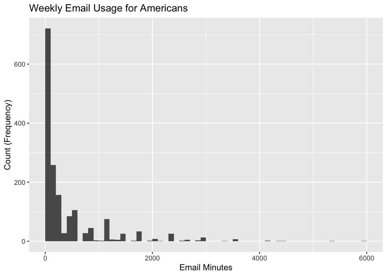
Question 2 continued… As we can see the distribution is very skewed to the right (positively skewed). Because of the way the arithmetic mean is calculated, large positive outliers (that are clearly present in this distribution) will produce a large, biased mean. In this instance, the median is probably a better “average value”, because it is not distorted by (biased to) the large positive outliers.
#Question 3 - Using the `infer` package, we calculate a 95% bootstrap confidence interval for the mean amount of time Americans spend on email weekly.

# Use the infer package to construct a 95% CI for delta
set.seed(1234)

boot_gss <- gss_email2 %>%
  specify(response = email) %>%
  generate(reps=100, type="bootstrap") %>%
  calculate(stat = "mean")

email_ci_1 <- boot_gss %>%
  get_confidence_interval(level = 0.95, type = "percentile")

#We work out the hours and remaining minutes so that we can present the confidence intervals in 'humanised' form...
Hours = email_ci_1 %/% 60
Minutes = email_ci_1 %% 60

email_ci_humanized <- c(Hours[c(1)], Minutes[c(1)], Hours[c(2)], Minutes[c(2)] )
email_ci_humanized <- as.data.frame(email_ci_humanized)

colnames(email_ci_humanized) = c("Lower CI Hours", "Lower CI Minutes", "Upper CI Hours", "Upper CI Minutes")
print(email_ci_humanized)
## Lower CI Hours Lower CI Minutes Upper CI Hours Upper CI Minutes
## 1 6 28.43919 7 28.86398This result seems fairly reasonable. The confidence interval perhaps seems fairly wide, given the large number of data points, but this could be due to the fact that there is large variation in the data, and that large positive outlying values (of which there are a few), will introduce bias and largely affect the mean.
Question 4 - Would you expect a 99% confidence interval to be wider or narrower than the interval you calculated above? Explain your reasoning.
We would expect the 99% confidence interval to be wider than the 95% interval. This is because the confidence interval is formulated using the Z/t level, which increases when you look for an interval of greater confidence. For example, the critical Z-value for a confidence interval of 95% is 1.96, but this value would be 2.58 for a 99% confidence interval. Because this critical value is multiplied by the standard error to form the confidence interval, we can expect the interval for 99% confidence to be wider. This is intuitive, because increasing the size of a given region naturally increases our confidence that the mean lies within this specified region/location.